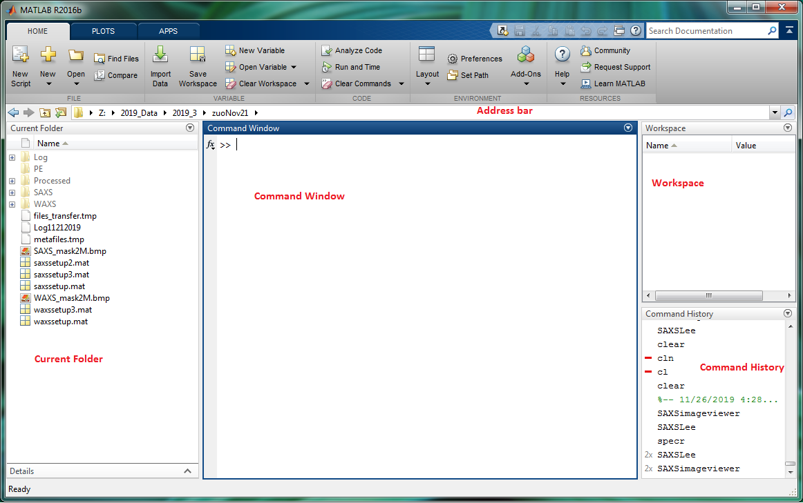
Double-click the Matlab icon at the Desktop, you will get the Matlab Window like Figure 1. From the Address bar, navigate to your data folder. In your Data Folder, you will have several folders, i.e., "SAXS" folder --for SAXS data; "WAXS" --for WAXS data; "PE" --for perkinElmer detector data; "Log" --log files for your image data measurements.
Figure 1. Matlab program window. "Current Folder" displays folders and files under your folder. You can run matlab functions and commands in "Command Window" . "Workspace" shows the matlab parameters in memory. "Command History" displays commands/operations run recently in "Command Window"; you can double-click the command to run it from the history list.
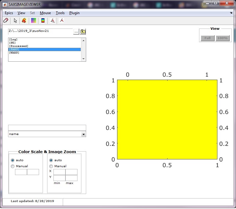
Figure 2A

Figure 2B
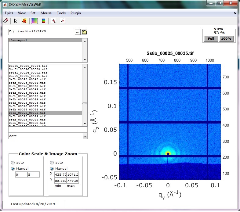
Figure 2C
Execute (type and hit enter) “SAXSimageviewer” in the matlab "Command Window" and you will get the matlab graphic window "SAXSIMAGEVIEWER" for 2D image visualization. The command could also be run in the “Command History” sub-window.
Choose an image data folder - for instance, "SAXS". Under menu "Plugin", click "Experiment Setup" - a matlab GUI program "GISAXSshop" will pop up. Images can be listed by "name", "date", "bytes", or "datenum". If listed by date, most recent ones stay at the top. Click any image file to display.
Click the square color icon to switch image color scales between log and linear scales. This can also be done through "View" menu. There are choices of "auto" and "Manual" for Color Scale at left bottom; "Manual" with range of [0, 5] is recommended.
There are two choices for Image Zoom - "auto" and "Manual". "auto" will display the whole image; "Manual" will show specified area. With the cursor on the image display, use the left mouse button to drag the image (pan motion), and use the right mouse button to zoom in/out.
Under menu "Epics", you can specify image data from which detector ("Pilatus2M", "PerkinElmer", or "Mar 300") will be automatically updated in the display window.
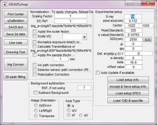
Figure 3. GISAXSshop/gisaxsleenew program screen
This program is needed for SAXSIMAGEVIEWER to correctly display 2D images.
To start it, click "Experiment Setup" from "Plugin" menu in SAXSIMAGEVIEWER, or execute “gisaxsleenew” from "Command Window" or "Command History".
Input parameters in "Experimental setup" section, or load them using "Load setup info" button if pre-saved info exists. After experimental setup information is available, the q_x, and q_y values will be computed and displayed in the 2D image window (Figure 2C). Then, the q value at every pixel will become available and ready to check using mouse cursor.
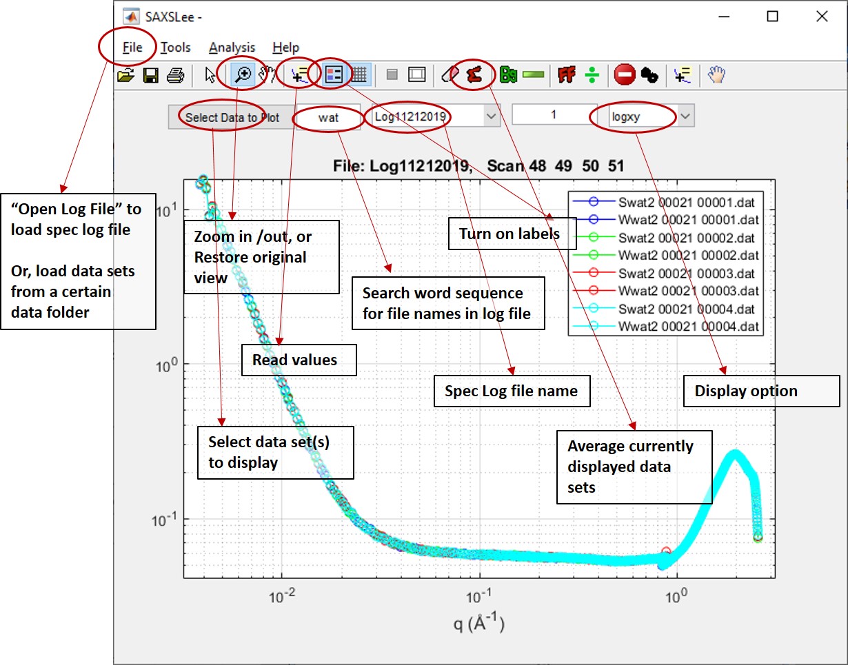
Figure 4. SAXSLee program GUI
To view the converted 1D profiles, type “SAXSLee” and hit "Enter" key in the main matlab "Command Window", and you will get the following GUI program screen.
Under the "File" menu, click "Open Log File..." to load the spec log file. The spec log file is starting with "Log", followed by the first experimental date, for example, "Log11212019".
Spec log file contains records of sample measurements and motor scans. Do NOT modify the spec log file! It may mess up data collection!
When the program loads the spec log file, it reads data file names from the spec log file. At 12-ID, 2D images will be automatically converted to 1D curvers. Both will be saved to your data folder. Now, you can start to look your 1-D data through "Select Data to Plot". The program screen also provides other functions, such as zooming, reading data point value, displaying options (linear, log), averaging, and subtraction.
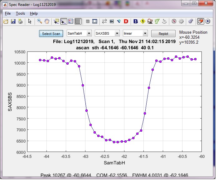
Figure 5. specr program GUI
To view the motor scan, type "specr" in the main matlab "Command Window", and you will get the following GUI program.
Under the "File" menu, click "Open Log File" to load the spec log file, then you can start to look your data through "Select Scan".